
Multimedia modelling of organic pollutants: The fugacity approach
Jamie Harrower
Glasgow Caledonian University / James Hutton Institute
[email protected]
ECG Bulletin July 2020
Glasgow Caledonian University / James Hutton Institute
[email protected]
ECG Bulletin July 2020
Organic Pollutants (OPs) have been a major concern for the environment for decades due to their persistence and toxicity. Up until the 1990s, non-polar hazardous compounds, persistent organic pollutants (POPs) (1), were priority pollutants and, as a result, intensive monitoring campaigns were conducted. These pollutants are still very important to monitor because of their detrimental ecological effects and persistence (long half-lives). In recent years, however, there has been more focus on emerging organic contaminants (EOCs) (2), which include pharmaceuticals, personal care products, pesticides and endocrine disrupting compounds (EDCs). EOCs and POPs enter the environment through various sources including wastewater treatment plants (WWTP), landfill sites, agricultural run-off and industry/hospital effluent.
Monitoring OPs in the environment can be challenging because of the considerable time and resources required to conduct field and lab work, and the complex matrices which can interfere with analysis. A selective extraction and clean-up step is required to ensure analytical instruments can detect contaminants at very low levels (ppb/ppt).
Concept of Fugacity
Compound fate in the aquatic environment can be determined using mathematical models known widely as fugacity calculations. The concept of fugacity was first developed by Lewis in 1901 (3). Then Donald Mackay applied this concept to multimedia models in environmental chemistry to describe the processes controlling the behaviour of chemicals in environmental media (4,5).
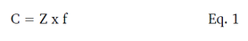
The term Fugacity describes a chemical’s escaping tendency (5). Therefore, when modelling compounds in the environment, fugacity describes the ability to move between two different environmental compartments. Equal fugacity is expected in both phases, as is the vapour pressure of the compound. The relationship between fugacity (f), concentration (C, molm) and fugacity capacity (Z, molmPa) is shown below (Eq. 1). The Z value is specific to a chemical and is dependent on the phase. A compartment with a higher fugacity capacity can accept a higher concentration of a given micropollutant.
Monitoring OPs in the environment can be challenging because of the considerable time and resources required to conduct field and lab work, and the complex matrices which can interfere with analysis. A selective extraction and clean-up step is required to ensure analytical instruments can detect contaminants at very low levels (ppb/ppt).
Concept of Fugacity
Compound fate in the aquatic environment can be determined using mathematical models known widely as fugacity calculations. The concept of fugacity was first developed by Lewis in 1901 (3). Then Donald Mackay applied this concept to multimedia models in environmental chemistry to describe the processes controlling the behaviour of chemicals in environmental media (4,5).
The term Fugacity describes a chemical’s escaping tendency (5). Therefore, when modelling compounds in the environment, fugacity describes the ability to move between two different environmental compartments. Equal fugacity is expected in both phases, as is the vapour pressure of the compound. The relationship between fugacity (f), concentration (C, molm) and fugacity capacity (Z, molmPa) is shown below (Eq. 1). The Z value is specific to a chemical and is dependent on the phase. A compartment with a higher fugacity capacity can accept a higher concentration of a given micropollutant.
Fugacity models become more complex as more data becomes available, and are assigned as different levels (1, 2, 3, 4). These calculations can also be applied various systems including quantitative water air sediment interactions (QWASI), sewage treatment plants (STP) and equilibrium criterion models (EQC). These will be described in more detail later. Chemicals flowing into a (dynamic) system, contained in water, sediment, biomass solids, and air, are driven by processes such as degradation and advection (more detail later). The rates of these processes can be described using D values (molhPa). In order to fully develop a fugacity mass balanced model, determination of D values is necessary. To determine D values, Z values are required, as well as specific information on the compounds being studied (physicochemical properties)/rate constants, and site-specific information on the STP, such as effluent discharge and size of STP. D values can be thought of as transport parameters, with units of molhPa.
Given the scope of multimedia modelling, this article will briefly discuss level 1, 2 and 3 models, and describe specific applications of fugacity models.
Partition Coefficient
Given the scope of multimedia modelling, this article will briefly discuss level 1, 2 and 3 models, and describe specific applications of fugacity models.
Partition Coefficient
A key parameter in fugacity calculations is Kow, the partition coefficient (Eq 2), which is derived from thermodynamics or can be measured experimentally.
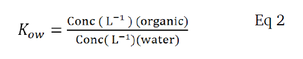
Octanol is chosen as the solvent because it provides suitable conditions as the organic layer, mimicking fatty/lipid biological tissues (6). In most cases, the partition coefficient is written as logKow, and measurements are taken of the neutral compound only in each layer. The shake flask method, outlined by the OCED guidelines (6), is a simple method to accurately measure logKow. A known concentration of compound is spiked into a system of specified ratios of octanol and water (which have been saturated with one another). The two layers are mixed thoroughly until equilibrium is obtained and allowed to separate. The aqueous layer is then carefully sampled and analysed using a technique such as High Performance Chromatography (HPLC) or UV-Vis Spectroscopy (7,8).
Ionisation of Organic Compounds
Compounds with ionising protons in their structure must be considered when using fugacity calculations. Charged structures can be formed at environmental pH levels which, in turn, can impact environmental partitioning. This is due to multiple acid dissociation constants and the wide range of physicochemical properties that some pharmaceutical drugs, such as antibiotics, pain killers and anti-inflammatories, contain. In contrast, non-polar compounds, such as polychlorinated biphenyls (PCBs), polyaromatic hydrocarbons (PAH) and polybrominated diphenyl ethers (PBDE) are also frequently found in the environment. Compounds such as these do not ionise at environmental pH values and, therefore, only one species (the neutral) of the compound is considered. PCBs have relatively high logKow values, and are described as hydrophobic, whereas antibiotics such as ciprofloxacin, have low logKow values (Figures 1-2). Therefore, their chemical behaviours will differ in-situ. Ciprofloxacin, unlike PCB-180, is able to form charged structures and zwitterions at environmental pH levels.
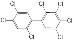
Figure 1. Chemical Structure of PCB-180
|
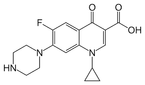
Figure 2. Chemical Structure of Ciprofloxacin
|
Level 1 Model - Closed System
A level 1 model describes a compound’s fate in the environment by making the following assumptions:
A level 1 model describes a compound’s fate in the environment by making the following assumptions:
- The system is closed, the volumes of the compartments are fixed, and the total amounts of chemicals distributed amongst the compartments are constant (Figure 3).
- The system is in an equilibrium steady state, meaning that the concentration of a chemical within a compartment is uniform, and the chemical potentials of a given species in different compartments are equal.
|
Calculations then determine the partitioning of chemicals between compartments labelled a, w and s (air, water, and sediment respectively) with volumes Va, Vw and Vs respectively. The respective concentrations Ca, Cw and Cs in each compartment can be used to calculate the partition coefficient (Kaw, Kws).
Level 2 Model – Dynamic Environment (equilibrium assumed)
A level 2 model describes a dynamic environment with inflows and outflows of chemicals through the compartment such that, at any given instant, the different phases are in equilibrium with one another (5). Partition coefficients can be used to describe the distribution of chemicals between the compartments. The main assumptions of a level 2 model are: |

Figure 3. Illustration of a simple 3-
compartment Level 1 model
|
- The system is open, meaning that, although the volumes are fixed, the total mass of chemicals distributed amongst those compartments may vary with time, or there may be equal inflows and outflows of chemicals that lead to steady state distributions.
- The distributions of chemicals amongst the compartments at any given instant is determined by the conditions of the chemical equilibrium and equilibrium partition coefficients, K, even if there is a throughput of chemicals.
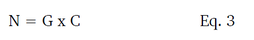
- Advection; a chemical is transported into or out of the region of interest by the flow of a supporting medium. The rate of advection (N = molh) (Eq. 3), is the product of the flowrate of the advecting medium (G = m3h) and the concentration of the chemical in that medium (C = molm) (5).
- Degradation and chemical reactions, which lead to a change in the total chemical within the region of interest.
Level 3 Model – Dynamic Environment (equilibrium not assumed)
Level 3 calculations include the transport by diffusive processes. For instance, a chemical takes time to diffuse within a compartment, driven by a concentration gradient. At equilibrium, the concentration profile is uniform and there is no net diffusion. This allows us to consider the introduction of some chemical at different rates into each compartment, which causes a non-equilibrium distribution of the chemical and, hence a net flow between them; this is intermedia transport. One study applied Level 3 fugacity calculations to predict the concentrations of antibiotics in a number of water basins in China (10). This study proved that the model was comparable with the available field data at specific sites.
Application of Fugacity models
Based on the theory of the fugacity calculations, researchers have developed many other models for systems. Among them are the EQC model, STP model and QWASI model.
The Equilibrium Criterion model
The EQC model was designed and based on evaluative level 1-3 fugacity models, described by Mackay et al. (11). It may be employed to systematically reveal general features of the behaviour of a chemical in a generic environment. The model enables progression through the sequence of levels 1-3 for a variety of chemicals. The model also separates chemicals into categories based on different properties including the ability to partition into different environmental compartments, volatility and water solubility (12). The chemicals are broadly divided into Type 1 (common pollutants – such as PCBs, PAHs), Type 2 (cations, anions and involatile chemicals), and Type 3 (long chain hydrocarbons, silicones and polymers). An important advantage of the EQC model is the ability to treat a greater range of chemicals than other models, but it is primarily utilised for non-polar species (12).
The Sewage Treatment Plant Model
The STP model was developed by Clark et al. (13), and is aims to understand the chemical behaviour and fate of contaminants in a conventional WWTP. The model is based on mass balances produced at each stage of the WWTP, which correlate and predict steady state phase concentrations, and process stream fluxes and the fate of micro pollutants. A limitation of this model is its inability to correctly model ionised compounds. As such, the model was upgraded to STP-EX, incorporating an ionic/neutral factor to upgrade Z values based on the compound under investigation, its pKa , and the pH of the wastewater (13). The STP and STP-EX model have been applied to conventional WWTPs all over the world, and used as a screening tool for risk assessments (14-16).
The Quantitative Water Air Sediment Interaction Model
The QWASI level 3 model was developed by Mackay and is used to predict contaminants behaviour in dynamic environments, such as rivers and lakes. Since its development, the QWASI model has been further modified (17). Based on fugacity calculation concepts, the model has been used to investigate a range of chemicals in lakes, and proved to be accurate compared to onsite measurements (18). Since its development, the QWASI model and modified versions have been applied to many studies to simulate the concentrations, distributions, transfer fluxes and bioaccumulation of chemicals in lakes and river systems (17-23).
D values and the fugacity are highly important in QWASI calculations. These are used to calculate rates of the contaminant (molh), where D values are calculated by multiplying G values (m3h) by the Z values(molmPa).
References
- Jones, K. C., and De Voogt, P., Environmental Pollution, 100 (1-3), 209-221 (1999).
- Petrie, B., Barden, R., and Kasprzyk-Hordern, B., Water Research, 72, 3-27 (2015).
- Lewis, G.N., American Academy of Arts & Sciences, 37 (3), 49–69 (1901).
- Mackay, D., Environmental Science & Technology, 13 (10), 1218-1223 (1979).
- Mackay, D., Multimedia Environmental Models: The Fugacity Approach, 2nd Ed., CRC Press Taylor Francis Group Florida, USA (2001).
- OECD/OCDE. OECD Guideline for the Testing of Chemicals, 107, 1–4 (1995).
- Harris, M. F., and Logan, J. L., Journal of Chemical Education, 91( 6), 915-918 (2104).
- Borrirukwisitsak, S., Keenan, H. E., and Gauchotte-Lindsay, C., International Journal of Environmental Science and Development, 3 (5), 460 (2012).
- Zhang, Z., et al., Science of the Total Environment, 515, 1-11 (2015).
- Zhang, Q.Q., et al., Environmental Science & Technology, 49 (11), 6772-6782 (2015).
- Nishimura, C., Japanese Journal of Biofeedback Research, 19 (6), 3–9 (1992).
- Mackay, D. et al., Environmental Toxicology and Chemistry: An International Journal, 15 (9), 1627-1637 (1996).
- Clark, B., Henry, G. L. H., and Mackay, D., Environmental Science & Technology, 29 (6), 1488-1494 (1995).
- Wang, J., et al., Chemosphere, 69 (11), 1802-1806 (2007).
- Thompson, K., Zhang, J., and Zhang, C., Chemosphere, 84 (8), 1066-1071 (2011).
- Küster, A., et al., Integrated Environmental Assessment and Management, 6 (S1), 514-523 (2010).
- Mackay, D., et al., Chemosphere, 111, 359-365 (2014).
- Mackay, D., and Diamond, M., Chemosphere, 18 (7-8), 1343-1365 (1989).
- Guo, J., et al., Science of The Total Environment, 657, 87-95 (2019).
- Xu, F. L., et al., Ecological Modelling, 252, 246-257 (2013).
- Whelan, M. J., Chemosphere, 91 (11), 1566-1576 (2013).
- Warren, C. S., et al., Water Research, 36 (17), 4341-4355 (2002).
- Mackay, D., and Hickie, B., Chemosphere, 41 (5), 681-692 (2000).